The following sections are descriptions of how to use the SPLAT-VO windows, hopefully these should only serve as reference material, the function of windows should be clear from their descriptions, balloon-help and context. Use a window’s Help menu to view its related page on-line.
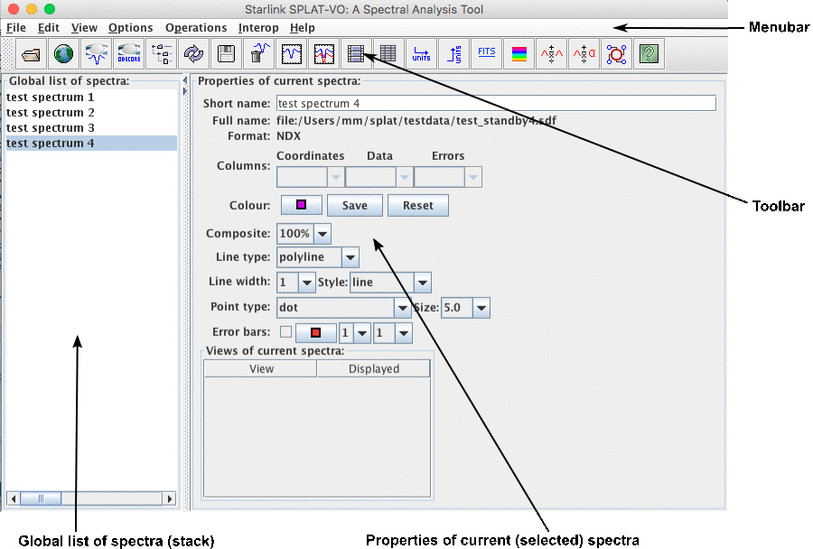
The browser window has several main elements, each of which is shown in the following figure:

Global list of spectra
In the Global list of spectra short names for each5 spectra are shown. The short
names are intended to allow the quick identification of spectra and can be modified
at any time by selecting the name and then typing a new name in the Short name
field (remember to press <Return> to make the change happen). Initially short
names are read from the TITLE or OBJECT properties of spectral data formats that
support these (i.e. NDF and FITS respectively), otherwise they default to the file
name.
Another important concept related to the global list, is using it to create a selected range or list of the spectra. Selection is important as this identifies which spectra you’d like to see properties for, or want to work with. There’s a quick tutorial on selecting spectra in the introductory material (§2.2).
Properties of current spectra
In the properties area there are controls for changing how the currently selected spectra are displayed (a spectrum always uses the same display properties) and where they are displayed.
If more than one spectrum is selected then the properties shown are those of the first spectrum (i.e. highest in the global list). However, any changes that you then make are applied to all the selected spectra.
If you load a table into SPLAT-VO the Columns: controls will show the names of the columns selected. If these are incorrect then you can choose a different set.
The properties that you can change include the colour (press on this to get a swatch of selectable colours), the composite value (that is the transparency so you can see lines or points through other line or points), the line type (simple connected polyline or histogram, or just a point marker). If you choose to draw lines then you can set the width and style (dashed etc.). If you choose to draw points then various types are available.
If the selected spectra have errors then you can display error bars by clicking on the Error bars: control. This is greyed out if errors are not available. The colour, number of sigma drawn and frequency of the error bars can be changed using the other controls on this line.
Views of current spectra
The views of the current spectra region shows the names of the plots that are displaying the currently selected spectra (this time if a plot is showing only some of the spectra, then it is highlighted in red). To add a spectrum or list of spectra to a plot, select their names in the global list and then click on the Displayed control (normally this results in a tick appearing). If a plot is already displaying some of the selected spectra then you force it to display them all by clicking twice – the first click removes the selected spectra and the second puts them all back, plus the ones not already shown.
To make a plot visible double click on its name. This should raise and deiconify it.
Toolbar and menus
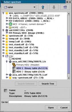
The toolbar region has a series of buttons that act as short-cuts to many of the functions found in the main menus. Here’s a quick break down of what they do:
guess (either on the command-line or by
using the open file dialogue).
all the spectra in the global list. Each time you press this button
a new random seed is used to generate a different sequence of colours, so keep
pressing until you see a sequence you like.
Interesting menu items not found in the toolbar are a list of standard line position catalogues (for optical and some IR and submillimeter lines), these are found in Options->Line identifiers. Others are to do with controlling the selection of the spectra and plots (see the Edit menu, just like deleting spectra from the global list you can delete all the selected plots) and changing the ‘look and feel’ of SPLAT-VO. These options are found in the Options->Look and Feel and Options->Colour Theme sub-menus. Note that if you select the CDE/Motif look and feel you cannot change the colour and fonts used.
You can also save and restore the global stack of spectra to and from diskfile using a special data format that is only recognised by SPLAT-VO. Using this method allows you to save a working set of spectra and restart an analysis later. Properties such as the line colours are restored, but any relationship between disk files and the spectra in the global list is lost. Data saved in a stack are compressed.
The Interop menu contains items for communicating with other SAMP-aware desktop applications. This is described in the Tool interoperability section (§6).
Finer control of the initial coordinate system picked by SPLAT-VO is given by the
Options->Find spectral coordinates menu item. When this is selected (the default),
SPLAT-VO will check for any spectral coordinate system in the input spectra and use that,
if the default coordinate system isn’t spectral. It will also use any units it can locate to
attempt a guess if all else fails. Unfortunately this means that if you intend to
view another coordinate system (like GRID to see the channel numbers), it
might fail, so switching this off gives you complete control. This option can
also be enabled using the -k,--keepcoords switches on the command-line.
Accelerator keys
The anatomy of a plot window is shown below:
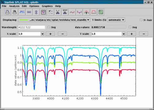
It has three main regions, the menubar & toolbar, the control panel and the display area.
The display area
The display area shows a view of all the spectra that are currently associated with this plot. The colours, plotting style etc. of these spectra are determined by their global properties as set in the main browser window.
The plot title and axis labels are determined using the properties of the current
spectrum, if possible. For instance if the current spectrum is an NDF then these
values are determined from the NDF’s title, units and axis components, or for more
recent NDFs from the properties of its WCS component. Similarly for FITS files
these values are determined using the world coordinates FITS keywords. To change
these look in the Configure Plot Options window, which is activated by pressing
the  button.
The size of the area used to display a spectrum is initially determined from an
automatic match of its data and coordinate extents to the visible surface of the
display area, you can change the size of the display surface using the zoom controls
described below and/or you can change the actual data limits using the Configure
Plot Options window. When you add or remove a spectrum the apparent size of
the display region stays the same and all the spectra now displayed are scaled to fit
within it. To return to a state where the visible surface matches the display area you
need to press the  and
and  buttons.
The Configure Plot Options window also offers the ability change the colour of the display area background, to draw the lines using anti-aliasing (which reduces the jagged effects, but at the cost of drawing speed), to modify the reserved area around the plot and do things like position the numeric labels, set the axis gaps etc.
The following interactions are provided in the display area.
If the vertical hair is enabled, then this also follows the mouse pointer.
The control panel
The control panel area provides controls for interacting with the plot. It also shows details of what spectra are displayed in the plot and a continuous readout of the X coordinate and corresponding data value.
The Displaying: drop down list shows the names and current rendering properties of any spectra that are displayed. If you choose a spectrum from this list it becomes the current spectrum and is used as the basis for the plot’s coordinates (so the readouts now show the values of this spectrum, also the plot will be re-drawn if the coordinate system of the newly selected spectrum is different). The selected spectrum also becomes selected in the browser window (so you see its details more clearly and apply modifications). This spectrum is also the one used by any tools (such as background and line fitting) that work with only one spectrum. If you remove this spectrum using the Edit->Remove current spectrum option then the next spectrum in the list becomes the current one.
The Y limits (%): drop down list provides a series of quick cuts for setting the limits of the Y axis. Normally this is the full range, but using a percentage cut can usefully clip the range to reject extreme outlier data values. The data values used are restricted to the limits of then X coordinates (all when automatic ranging is used, the default ).
The Wavelength: entry control has two functions. The first is to show the current
wavelength. The second is to allow you to centre the display area on a specific
coordinate. Just type in the value you want to see here and press <Return>. Note
that the label of this area modifies to match the label of the X axis, so could say
something different to Wavelength:.
The :V-hair checkbox controls whether the ‘vertical hair’ is shown. The vertical hair is just a vertical line that follows the mouse pointer around the display area. It can be quite slow, so isn’t shown by default.
The X scale: and Y scale: controls change the zoom of the display area. The plus
and minus controls increase and decrease the zoom by one, or you can choose a
zoom from the drop-down lists, or you can type in a decimal value (which should
be greater than equal to one) and press <Return>.
The :log controls determine if either of the axes are drawing using log spacing (this is not possible if either axis spans the value zero). Finer control of the log spacing and labelling can obtained using the plot configuration window.
The Track free checkbox determines what values are shown in the continuous coordinate readouts. When unchecked (the default) the values shown are the nearest ones of the current spectrum to the pointer position. When checked the readouts show the coordinates under the pointer.
Toolbar and menus
The toolbar region has a series of buttons that act as short-cuts to most of the functions found in the main menus. Some of these create new windows with complex actions that should be consulted for further help.

Cut <n> of <current_shortname>. This facility is
useful to create printouts of just parts of a spectrum and to speed up processing of
very large spectra.
The Options menu contains several control items whose values are preserved between invocations of SPLAT-VO.
Whether this works or not depends on whether the spectra that you have read
in contain correct descriptions (or descriptions that SPLAT-VO can make good
guesses about) of the spectral coordinates and data fluxes and whether the
flux system is supported. If this doesn’t work then check that your spectra
have valid descriptions using the toolboxes in the main browser window for
inspecting and setting spectral coordinates and data units ( and
and  ).
).
In the case of line identifier catalogues, these will also be transformed to the rest frame of the observed source (i.e. they will be red or blue shifted if you have defined the source velocity as part of its coordinate system definition).
This option is switched on by default. If your spectra do not need aligning switch if off for extra performance.
The items possibly included in the synopsis are:
These are somewhat tuned for submillimetre observations at the JAC and for spectra extracted by GAIA from cubes, so many may be missing for spectra from other sources. Names in parenthesis are either the FITS keywords or AST attributes used to obtain the values.
The Graphics menu
The Graphics menu provides methods for drawing text and a range of figures on the plot. This allows you to add annotations, but also provides the basis for the interactive graphics used by the various toolboxes.
To draw a figure on a plot you need to select an option from the Drawing mode sub-menu and then, depending on the figure type, either drag out a region or select fiducial points. When creating a figure using points these are completed using a double click on the last point.
In the Drawing mode menu the currently available figure types are:
There are also two special modes:
When the mode is select (this is usually the default state), clicking on a figure selects it. You can then
drag it around to move it, or drag one of the grips (the little squares) to change the shape. To select
more than one figure you hold down the <Shift> while clicking.
The edit mode can be used to add new points to a polyline, polygon or interpolated curve. Just select this, click on the figure you want to edit and then start adding new points. You can also edit text strings, just choose the edit mode and click on the text, this produces a dialogue with the text for editing.
To change the properties of a figure (line width, fill/outline colour, font etc.) just select the figure and then choose the option you want to change from the various menus. You can define these before creating a figure too.
Interpolated curves are like polylines in that they are defined by a series of points, but they can only have increasing or decreasing X coordinates (so cannot double back on themselves). They are intended for drawing figures that are related to spectra, specifically spectral backgrounds and lines. In fact if you draw an interpolated curve you can convert it into a spectrum for removing from a real spectrum using the Generate spectra from interpolated lines toolbox. The types of interpolation scheme available are:
Once you have created your figures you may want to save them for restoration at a later time, this can be done using the Graphics->Save/restore figures dialogue. Figures are saved using the physical coordinates of the spectrum, so should be re-drawn at the correct wavelengths etc. on new plots.
Accelerator keys
This window provides access to the Virtual Observatory (VO). Using it you can search a region of sky for spectra or search for spectra associated with a specific astronomical object. Once you have done that you can then download all or some of these spectra for display and analysis in SPLAT-VO.
In the VO spectra are made available by SSAP servers (SSAP stands for Simple Spectral Access Protocol) and using this window you can also select which of these servers you want to query. That is important if you are only interested in spectra covering specific wavelengths or types of observations. These searches can be further refined using additional parameters like a range of wavelengths or times. Addtional Optional Parameters are also provided for even more refinement, but note that these may not be supported by all SSAP servers.

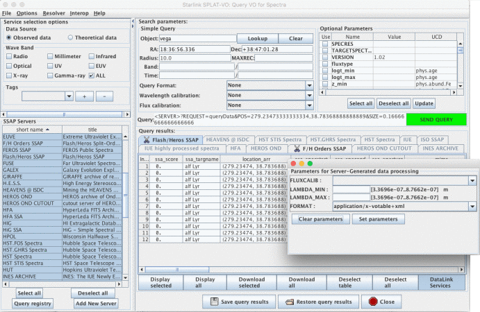
The figure above shows the window after a query has been made. The window is divided in three main areas. The left area is the SSAP server selection area, where the current list of SSAP servers is shown and also options to select a subset of servers to be queried. The upper right area is the query parameters area, where query options can be entered. The right-lower part is the results area, showing the query results.
Server selection
You can select one or more servers from the SSAP Servers list by clicking on them. It’s also possible to select a subset of servers based on their given metadata. Selection can be made according to data source (observation or theory data), and waveband. It’s also possible to add tags to one or more servers, so only the tagged servers will be queried if the tag is selected. When right-clicking on a server in the SSAP Servers list you get a popup menu containing options to tag, to remove, or to see information on the service. To add a new SSAP server, which is currently unknown to the VO, to the current server list, click on the Add New Server button. A new window will open where the information about the new server can be filled in. The Query registry allows you to query a VO registry for a list of all the SSAP servers it has registered.
SSAP query
To lookup the coordinates of an object just type in an identifier in the Object field and either press
<Return> or the Lookup button. Alternatively if you know the coordinates (FK5/J2000) of the region
of sky you can just enter the coordinates in the RA and Dec fields. It is also possible to query the
servers about an object by name, useful for solar system work, in that case just enter a name and leave
the RA and Dec fields empty.
The Radius value is a number of arcminutes to search about the position. The Band entries define a lower and upper limit, in meters, for the spectral bandpass (not all SSAP servers support this option, those that do may offer just an upper limit and allow you to set a wavelength to include by setting just a lower limit). The Time entries define either a time that should match the time the spectra where taken, or a range in which they should match (again not all servers support this option). The MAXREC field will define the maximum number of spectra that will be retrieved from each selected service. The file format, wavelength and flux calibration options can also be chosen. If the value is "None", the query will not contain these parameters.
Besides the mandatory parameters, some servers also support a set of other metadata parameters. The Optional Parameters panel shows the metadata parameter supported by at least one of the selected services. The checked parameters having a non empty value field will be added to the query.
Once you have identified the region to search or object press the green SEND QUERY button to contact the current list of SSAP servers. To make these queries it may be necessary for you to tell SPLAT-VO about your local web-proxy server (this is the same as that you use in your Internet browser), select the Options->Configure proxy... item to do this.
Query results
Once the SSAP query is complete lists of spectra that the servers hold will be shown in the Query results: region. There is a tab of results for each server. If no tab has been created for a selected server, then the server has no spectra for the selected region or is not available at the moment.
When right-clicking on a spectra, a popup menu will appear. From this menu you can download or display the spectrum, see its fields (and, if supported, see a preview), or copy the contents of the current table, line or cell to the clipboard.
The next action is to select which spectra you want to download and view in SPLAT-VO. If you press Display all then all the spectra from all the servers will be downloaded and displayed in a single plot. Clearly this may take quite sometime if there are many spectra, so you can also download and display a subset. To do this select the rows that contain the spectra that you want to see (you can extend selections by using the control and shift keys while selecting a row and you can select spectra from more than one tab at a time) and then press the Display selected button.
Once the spectra have been downloaded they should appear together in a single plot. If this isn’t the case then some of the spectra are probably invalid and you will need to add them to a plot yourself (see the section on displaying more than one spectrum). If you want SPLAT-VO to match the coordinate systems and fluxes of the spectra then make sure that the Options->Match coordinates and/or fluxes item is still switched on in the plot window.
To view a single spectrum quickly just double click on its row. This will download the spectrum and
display it in its own plot window.
Server-side manipulation with DataLink
SPLAT-VO supports server-side manipulation through DataLink. After a SSAP Query is sent,
SPLAT-VO checks the responding servers for DataLink parameters, and marks them with a symbol
( ). If at least one DataLink supporting server has been found, a DataLink button will
appear below the query results. By clicking on it, DataLink. will be activated, and all results
tabs will be deactivated except the results from servers that support DataLink. When you
choose one of the active services, a window will appear, where the respective parameters for
sever-side manipulation can be entered. The parameters will be set by clicking on the set
parameters button. While dataLink is activated and the parameters are set, the spectra you select
and display or download will be manipulated using the chosen parameters. To deactivate
dataLink and have retrieve the original spectra just click on the dataLink button again.
Implementation status
SSAP is a protocol being developed by the IVOA (International Virtual Observatory Alliance1).
Currently spectra returned from SSAP servers may only be in basic formats, that is simple FITS and VOTables (partially some SED data model serialisation). However, the SPLAT-VO data model includes errors as well as coordinates and data values.
Support for spectral coordinates is provided by the Starlink AST library (SUN/211) using an implementation of the FITS-WCS paper III Representations of spectral coordinates in FITS (Greisen, Valdes, Calabretta & Allen). AST also provides the flux and data value conversion utilities used by SPLAT-VO which is based on interpreting the units strings system described in FITS-WCS paper I Representation of World Coordinate in FITS by Greisen & Calabretta. Conversion between fluxes is currently restricted to flux per unit wavelength and flux per unit frequency is provided and does not require any ‘dimensional analysis’ information to be present, just correctly formed units strings.
Server metadata information is provided by the respective maintainers, and may not be complete or accurate.
Accelerator keys
Besides SSAP, SPLAT can also query VO services supporting ObsCore (Observation Data Model Core) components via TAP (Table Access Protocol). This services are known as ObsTAP services. There are two ways of doing that in SPLAT-VO by using a cone search interface, like the SSAP query, or by sending an ADQL query. ADQL stands for Astronomical Data Query Language, based on SQL. There are introductions and tutorials for ADQL for instance at http://docs.g-vo.org/adql (Markus Demleitner) or http://is.gd/ADQLTutorial (Simon Murphy).
Server Selection The server selection interface works in the same way as the server selection in the SSAP window. Just that the servers list contains ObsTap services instead of SSAP services, and there are no optional parameters, as all parameters can be queried using TAP.
Simple Search The simple search interface uses the same parameters as the SSAP cone search, with the same functionality.
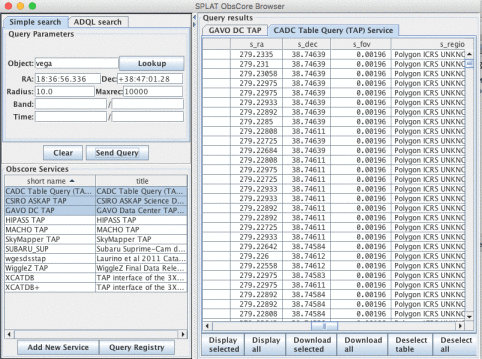
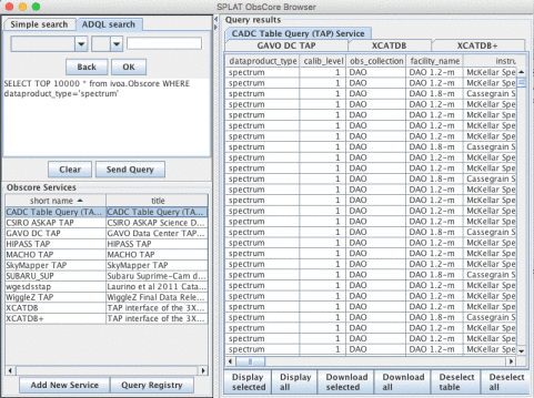
ADQL Search The ADQL search is more flexible and more powerful than the simple cone search. The main part is a text area, which can be edited. The beginning of the query
will get the first 10000 spectra from the selected servers. The TOP value may be changed to another value, if necessary. This query should be then refined or completed, either by choosing the parameters and expressions from the options provided (which will create a simple query) or by editing directly the the text area. Please refer to the ObsCore standard for the available parameters. (http://www.ivoa.net/documents/ObsCore/).
Implementation status
ObsCore and TAP are being developed by the IVOA (International Virtual Observatory Alliance2).
This window allows you to display a series of spectra from the global list, one after the other. It is possible to display these into an existing plot, that may already be displaying other spectra you’d like to use for comparison, or you can use a new plot.
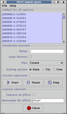
With careful control of the plotting options you can display into a plot with fixed data ranges, or see each spectrum plotted as autoscaled.
It is also possible to use this window to generate a series of JPEG or PNG images that you could combine into a movie of some kind.
Global list of spectra:
As in the browser window this is a view of the spectra currently stored in the global list. Initially all the spectra in the list are selected, but you may modify which spectra to animate by creating your own selection (reminder: the combination of shift-left-mouse click selects the range between the last selected row and the current position, and the combination control-left-mouse click, either adds the current row to the selection, or removes it, if already selected).
Animation controls:
The Delay: field accepts a decimal number of seconds to pause between displaying
the selected spectra. You can modify this during an animated sequence by pressing
the <Return> key.
The Loop forever: checkbox determines whether the animation sequence is restarted when all the selected spectra have been displayed. If set then you need to press the Stop button to stop the animation.
The Plot: drop-down list contains a list of all the currently available plots and the
special entry Create. If the Create option is chosen then a new plot will be created
to display the animation, otherwise the animation will take place in the selected
plot.
The Scaling option: radio buttons control how a spectrum is scaled when it is displayed.
The Current spectrum label just displays the name of the spectrum currently being added to the target plot. This information is repeated in the plot itself as the spectrum becomes the current one in the plot and is named in the Displaying: label.
The Start, Pause and Stop buttons do what is expected.
Capture controls
The capture controls are for creating a series of JPEG or PNG images of the plot as it
displays each spectrum. To enable (after getting the required effect using the Animation
controls) just click on the Start capture: check box. The output file names will
start with what name you type into the Basename for graphics files: entry
and have an integer number appended, plus the file type .jpg or .png. So a
default sequence would be SPLAT0.jpg, SPLAT1.jpg, SPLAT2.jpg,... You’ll then
need to find some software to convert these into a movie. The ImageMagick
convert command (when suitably configured) will convert these files into an
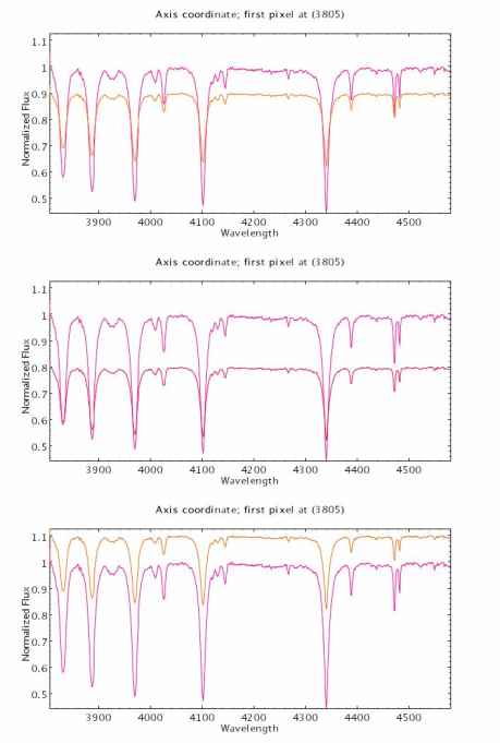
MPEG or animated GIF. The image below was created with the command (note
that the images were also scaled – view the html documentation or the pdf
documentation in a viewer that supports animation such as Adobe Reader to see the
animation.):
Accelerator keys
The purpose of this window is to allow you to see the actual data values of a spectrum and to make modifications to them. The spectrum being shown has it basic details at the top of the window and the values of the spectrum are shown in a table area that you can scroll.
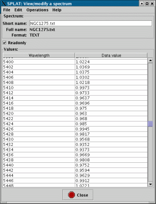
Modifications
If you want to modify any of the values, then you need to have a spectrum that isn’t
readonly. Spectra read from files always have readonly values, so this will generally
be the case. The simplest way to get a modifiable spectrum is to untick the Readonly
control. This will make a memory copy of your spectrum, enter this on the global
list and then load it into this window replacing the previous spectrum. The new
spectrum will be called ‘Copy of <oldname>’.
Note that if you want to plot this new spectrum you’ll need to go back to the main window and do this yourself (plots of the spectrum that this is a copy of are not going to show any modifications that you now make!).
Editing single values
To change a single value of any kind you can now just select the table cell (usually
by double clicking on it) and type in the new value. Press Return to make the edit
happen (this should immediately be shown in any plots of this spectrum).
Editing whole columns
You can make global changes to a whole column of values using special dialogues that either offer special functions (linear transformations), or allow you to define an algebraic expression (in terms of the existing values or a simple index counter starting at 1 for the first row).
Editing the data values column
To apply a global edit to the data values column you need to select the Operations->Modify data column item. This should produce a new window.
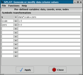
In which you can see an example expression , with the value set to and the zero value to . A list of preset expressions that should be generally useful is found in the Functions menu.
Naturally if you applied this expression then the data values would stay the same. A more complex example is shown next.
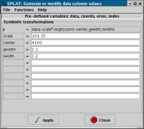
This presents the possibility of subtracting a single Voigt profile (the top part of this is greyed out as Voigt is a built-in function that cannot be represented as an algebraic expression).
If you need to use an expression of your own you might like to view the full list of functions that are available in the MathMap section of the KAPPA SUN. A lot of C-like intrinsics are available (abs, atan/sin/cos, tan/sin/cos, log, pow sqrt, etc.), which can operate on the data columns , and , as well as the virtual column.
Editing the error values column
Editing the error column is much like editing the data column, except that you can actually create a new error column, see the Operations->Modify error column item.
The error column can also be deleted using the Edit->Delete error column item.
Editing the coordinates column
Globally editing the coordinates can be done using the Operations->Modify coordinate column window.
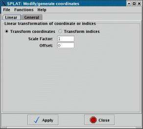
A simple built-in option of applying a linear transformation is offered (useful for when the coordinates are in fact some index related to wavelength). Under the General tab you can use algebraic expressions like those for modifying the data columns.
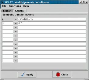
In this case the pre-defined expression for blue-shifting a spectrum in some wavelength units is shown.
Note: when you modify coordinates either singly or as a column any coordinate system information will be lost. If you want to retain this you’ll either have to re-enter this information or use the conversion facilities of the Coordinate system attributes window (using this other window you can transform between apparent place, Earth to Sun to Local Group etc. and to a source rest frame that has a velocity in a given direction, so you can correct for red/blue shift that way, in fact this is the recommended way).
Undoing and redoing changes
Using the Edit menu in the main view/modify window you can undo and redo any modifications that you make to the spectrum. The changes are propagated immediately so you can see these effects in any plots of the spectrum.
Accelerator keys
This window allows you to define the coordinate systems that describe your spectra. The most trivial use of these is simply to document what type of coordinate and units your spectra are measured in, examples are wavelength in air in angstroms, frequency in GHz, velocity in km/s, etc. When supplied these values will be used to annotate any plots, but can also be used to compare spectra in different coordinate systems and to transform a spectrum from one coordinate system to another.
A more complete description of the coordinate system also includes two further pieces of information, the time and place when the observation was made and the direction and speed of what was being observed. Taken together these define the ‘rest frames’ of the observation and the source.
In the following picture you can see that I have an observation (topocentric) of NGC1275 (RA: 03:19:47.49, Dec: 41:30:40.5 FK5 J2000) made in air, calibrated in angstroms, taken in June 1999 on the William Herschel Telescope. I’ve also entered that NGC1275 as observed from the centre of the Sun (heliocentric) has a recessional (relativistic) velocity of 5300km/s. Alternatively if you know the necessary redshift you can enter that value by selecting a Source system of Redshift (other possibilities are radio velocity, optical velocity and beta factor).
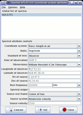
To apply this to a spectrum that has no coordinate information (or incorrect coordinate information) you need to press the Set button. Note that you can apply the same coordinates to more than one spectrum by selecting them all in the view of the global list shown in this window.
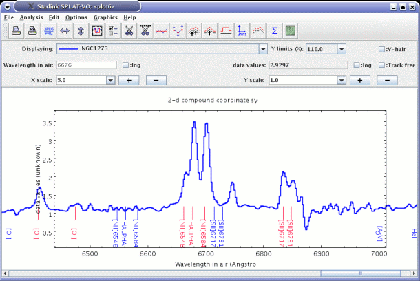
Now say that you wanted to compare this spectrum with a standard set of emission lines, obviously taken at rest in a laboratory. If you load the emission line catalogue and display it in the same plot (making sure that the Options->Match coordinates and/or fluxes item is switched on) the labels will be red-shifted to the rest frame of the source (i.e. where the lines from the galaxy originated). This is shown in action in the next figure where the lines before matching are shown in blue and red after matching.
The alternative to this method is switch Options->Match coordinates and/or fluxes off and transform the galaxy spectrum to what it would have looked like in the source standard of rest (i.e. if you had taken the measurements travelling with the galaxy). To do this change the Standard of rest: to Source but now press the Convert button. This remaps the spectral coordinates permanently.
Using this method you can also transform your spectrum to other systems and units (say frequency or energy) and rest frames (so you can go from topocentric to heliocentric or the kinematic or dynamic local standards of rest). With Options->Match coordinates and/or fluxes switched on you can also directly compare spectra calibrated in all these different systems.
When transforming to velocity (optical, radio and relativistic velocities are supported) a rest "frequency" is also needed. Conceptually this is the value that the centre of a line with locally zero velocity has. The rest frequency can actually be specified in various units, for instance angstroms.
The Spectral origin value is used when you want to draw spectral coordinates in some offset system. This value defines the zero point. It must be specified in the same units as the spectrum.
To find out more about spectral coordinate systems you’ll need to refer to ‘FITS-WCS paper III Representations of spectral coordinates in FITS (Greisen, Valdes, Calabretta & Allen)’ and the Starlink AST library documentation (SUN/211).
Accelerator keys
This window allows you to inspect, set or convert the units of the data values of your spectra.
The most trivial use of these is simply to document what type of units your spectra are measured in. However, a more powerful use of data units can be made when displaying more than one spectrum in a plot. In that case you can request that the data values of all the spectra are transformed into the same system, so you can compare values in Janskys with those in other flux per unit frequency and per unit wavelength systems (note to activate this option you must have the Options->Match coordinates and/or fluxes menu item selected in the plot window). For instance all the following systems are understood as fluxes and can be intercompared:
| Jy | () |
| W/m^2/Hz | () |
| W/m^2/Angstrom | () |
| W/cm^2/um | () |
| erg/cm^2/s/Hz | () |
| erg/cm^2/s/Angstrom | () |
Plus variations like
instead of
or maybe ,
etc. When reading unit strings like W/m^2/Hz you should say Watts per metre squared per Hertz,
which is actually mathematically the same as the expressions shown in to the right in parentheses
( in this
case). Note that dimensionally equivalent unit strings to those above maybe be recognised and
re-formatted.
In addition to flux systems dimensionally similar ones can also be used and transformed between in a plot, things like temperature. SPLAT-VO understands that and are temperatures in Kelvins and milliKelvins, same for units like and .
The units are described using strings that follow the conventions in FITS-WCS paper I Representation of World Coordinate in FITS by Greisen & Calabretta, and processed by the Starlink AST library (SUN/211). The following section is copied from SUN/211 for convenience. Not all units are relevant to data values (AST also provides the underlying coordinate transformations used in SPLAT-VO) and as noted above not all possible unit strings can be understood as fluxes (although support for more types is expected, for instance temperatures and magnitudes).
The adopted syntax is that described in FITS-WCS paper I Representation of World Coordinate in FITS by Greisen & Calabretta. We distinguish here between “basic” units and “derived” units: derived units are defined in terms of other units (either derived or basic), whereas basic units have no such definitions. Derived units may be represented by their own symbol (e.g. “Jy”—the Jansky) or by a mathematical expression which combines other symbols and constants to form a definition of the unit (e.g. “km/s”—kilometres per second). Unit symbols may be prefixed by a string representing a standard multiple or sub-multiple.
In addition to the unit symbols listed in FITS-WCS Paper I, any other arbitrary unit symbol may be used, with the proviso that it will not be possible to convert between spectra using such units. The exception to this is if both spectra refer to the same unknown unit string. For instance, an axis with unknown unit symbol "flop" could be converted to an axis with unit "Mflop" (Mega-flop).
Unit symbols (optionally prefixed with a multiple or sub-multiple) can be combined together using a limited range of mathematical operators and functions, to produce new units. Such expressions may also contain parentheses and numerical constants (these may optionally use “scientific” notation including an “E” character to represent the power of 10).
The following tables list the symbols for the basic and derived units which may be included in a units string, the standard prefixes for multiples and sub-multiples, and the strings which may be used to represent mathematical operators and functions.
| Basic units | ||
| Quantity | Symbol | Full Name
|
| length | m | metre |
| mass | g | gram |
| time | s | second |
| plane angle | rad | radian |
| solid angle | sr | steradian |
| temperature | K | Kelvin |
| electric current | A | Ampere |
| amount of substance | mol | mole |
| luminous intensity | cd | candela |
| Prefixes for multiples & sub-multiples
| |||||
| Sub-multiple | Name | Prefix | Sub-multiple | Name | Prefix
|
| deci | d | deca | da | ||
| centi | c | hecto | h | ||
| milli | m | kilo | k | ||
| micro | u | mega | M | ||
| nano | n | giga | G | ||
| pico | p | tera | T | ||
| femto | f | peta | P | ||
| atto | a | exa | E | ||
| zepto | z | zetta | Z | ||
| yocto | y | yotta | Y | ||
| Mathematical operators & functions
| |
| String | Meaning
|
| sym1 sym2 | multiplication (a space) |
| sym1*sym2 | multiplication (an asterisk) |
| sym1.sym2 | multiplication (a dot) |
| sym1/sym2 | division |
| sym1**y | exponentiation ( must be a numerical constant) |
| sym1^y | exponentiation ( must be a numerical constant) |
| log(sym1) | common logarithm |
| ln(sym1) | natural logarithm |
| exp(sym1) | exponential |
| sqrt(sym1) | square root |
| Derived units | |||
| Quantity | Symbol | Full Name | Definition
|
| area | barn | barn | 1.0E-28 m**2 |
| area | pix | pixel | |
| area | pixel | pixel | |
| electric capacitance | F | Farad | C/V |
| electric charge | C | Coulomb | A s |
| electric conductance | S | Siemens | A/V |
| electric potential | V | Volt | J/C |
| electric resistance | Ohm | Ohm | V/A |
| energy | J | Joule | N m |
| energy | Ry | Rydberg | 13.605692 eV |
| energy | eV | electron-Volt | 1.60217733E-19 J |
| energy | erg | erg | 1.0E-7 J |
| events | count | count | |
| events | ct | count | |
| events | ph | photon | |
| events | photon | photon | |
| flux density | Jy | Jansky | 1.0E-26 W /m**2 /Hz |
| flux density | R | Rayleigh | 1.0E10/(4*PI) photon.m**-2 /s/sr |
| flux density | mag | magnitude | |
| force | N | Newton | kg m/s**2 |
| frequency | Hz | Hertz | 1/s |
| illuminance | lx | lux | lm/m**2 |
| inductance | H | Henry | Wb/A |
| length | AU | astronomical unit | 1.49598E11 m |
| length | Angstrom | Angstrom | 1.0E-10 m |
| length | lyr | light year | 9.460730E15 m |
| length | pc | parsec | 3.0867E16 m |
| length | solRad | solar radius | 6.9599E8 m |
| luminosity | solLum | solar luminosity | 3.8268E26 W |
| luminous flux | lm | lumen | cd sr |
| magnetic field | G | Gauss | 1.0E-4 T |
| magnetic flux | Wb | Weber | V s |
| mass | solMass | solar mass | 1.9891E30 kg |
| mass | u | unified atomic mass unit | 1.6605387E-27 kg |
| magnetic flux density | T | Tesla | Wb/m**2 |
| plane angle | arcmin | arc-minute | 1/60 deg |
| plane angle | arcsec | arc-second | 1/3600 deg |
| plane angle | mas | milli-arcsecond | 1/3600000 deg |
| plane angle | deg | degree | pi/180 rad |
| power | W | Watt | J/s |
| pressure, stress | Pa | Pascal | N/m**2 |
| time | a | year | 31557600 s |
| time | d | day | 86400 s |
| time | h | hour | 3600 s |
| time | yr | year | 31557600 s |
| time | min | minute | 60 s |
| D | Debye | 1.0E-29/3 C.m | |
Accelerator keys
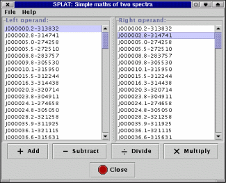
This window allows you to add, subtract, divide and multiply two spectra. To use it just select a spectrum in the Left operand: list and a spectrum in the Right operand: list. Now select the operation you want to apply between them. A new spectrum called:
Sum: (short name of left operand) + ( short name of right operand)
Diff: (short name of left operand) - ( short name of right operand)
Ratio: (short name of left operand)
( short name of right operand)
Product: (short name of left operand) x ( short name of right operand)is created on the global list.
Note: the algorithm used to combine spectra that do not have the same wavelength positions is a simple interpolation. This does not preserve total flux, or errors, so this tool should only be used for quick qualitative arithmetic between real spectra. Artificial spectra (such as polynomial fits) do not have this restriction.
Accelerator keys
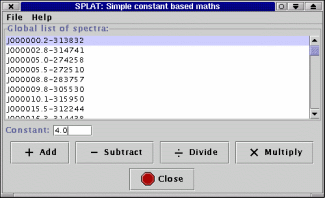
This window allows you to add, subtract, divide and multiply a spectrum by a constant. To use it just select a spectrum in the Global list of spectra: and enter the value you want in the Constant: entry area. Now select the operation you want to apply. A new spectrum called:
Sum: (short name of spectrum) + (<constant>)
Diff: (short name of spectrum) - (<constant>)
Div: (short name of spectrum)
(<constant>)
Mult: (short name of spectrum) x (<constant>)is created on the global list.
Accelerator keys

This window always shows a full view of the spectra displayed in the related plot. It is designed to
allow you to pan around the full sized view by moving the red rectangle.
The display is always drawn at the same aspect ratio as the full sized display, but is scaled to fit within the width or height of the panner window. Because of this there may be better widths or heights to fit any particular zoom. Resize the window to gain familiarity with this feature.
The following mouse interactions are provided:
Centre display area, to centre the display area just put the mouse pointer over the
panner and press the left mouse button.
Scroll display area, to scroll the display area you need to drag the red rectangle. To
do this just place the mouse pointer in the red rectangle and then press the left mouse
button down, now move the mouse to drag the rectangle. When you’re finished release
the mouse button.
Zoom display, to zoom the main display by a factor of 1 in X, just press the middle mouse
button.
Unzoom display, to unzoom the main display by a factor of 1 in X, just press the right
mouse button.
Accelerator keys
This window provides a series of paged controls for configuring the plot display area. This help section describes each page in turn. Global options that apply to the configuration window as a whole are the ability to Auto-update any changes to what the display area is showing and to save and restore configurations to and from an XML storage system.
Normally configuration changes happen immediately as Auto-update is switched on by default. If you prefer to wait for changes then you will need to press the Draw button. You also need to press the Draw button when making changes to the data limits (these may not be in a valid state until you’ve entered the complete coordinate value).
Accelerator keys
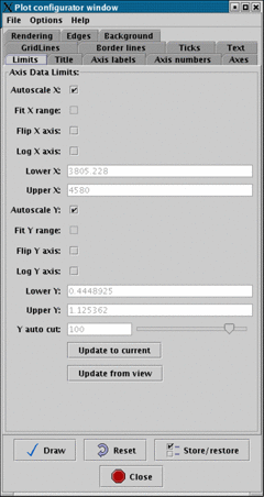
This page allows you to set the physical limits of the axis drawn in the display area. The default configuration auto-scales all spectra to fit within the currently available display area.
If you want to apply limits of your own then, untick the auto-scale checkboxes and enter your values in the lower and upper entry areas. Remember to press Draw to apply the limits.
You can also get either axis to display itself using logarithmic scaling (if possible, there are limitations, like not being able to contain the coordinate zero) and to display the axes ranges flipped top to bottom or left to right.
Other useful options are the checkboxes Fit X range: and Fit Y range: that also make the ranges that you supply fit the visible display area exactly (these are like the fitwidth and fitheight options in the plot window) and Y auto cut: which applies limits to the Y axis using percentile cuts (the data used to estimate the limits lies within the current X coordinate range).
The Update to current button sets the X and Y limits to those of the full plot (these are the values shown initially). The Update from view button sets the X and Y limits to those of the visible part of the display area. This is useful to just show coordinate axes for what you can see.
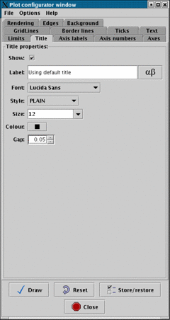
This page allows you to change the title shown in the plot. Using the controls you can define the
font, style, size, colour and gap, from the nearest axis, of the title. You can also decide to
have no title shown and insert any character from the chosen font (depends on the font,
but usually these include the Å sign, press the  button to see the character selection
window).
The text shown in the Label: field is an accurate rendering of what is shown in the plot window. The
default title can be restored by setting the text of this field to blank, or to the text Using
default title (this text is used so that you can see the result of any changes you’re about to
make).
Superscript and subscripting are available using AST Escape sequences, for instance:
| AST escape sequence | result |
| super%^100+script%^+ | |
| sub%v100+script%v+ | |
| %% | |
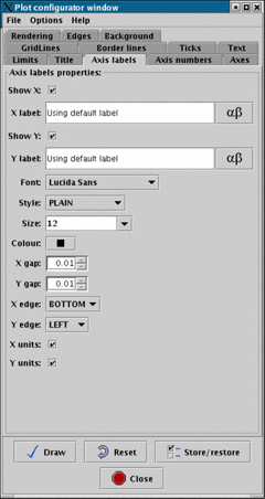
This page allows you to set the labels used on the X and Y axes. It also allows you to choose the font, style, size and colour used, as well as how far to position from the axis, which axis to attach to and whether to include any units (as a string in parenthesis). The text shown is an accurate rendering of what is shown in the plot window.
As with the title you can insert any characters from the font, and use AST Escape sequences to get effects like super and sub-scripting.
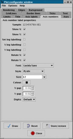
This page allows you to configure how the axis number labels are rendered. As with other pages you can define the font, style, size and colour used, as well as the separation between the actual axes and the labels. An accurate rendering of how the labels will be drawn is shown in the Sample: label.
The Set log labelling: option controls whether the numbers are drawn using an exponent notation. This is the default if log spacing has been selected for the axis (so you can also use this to not get exponent labelling when the axes are drawn using a log scale).
The Digits: drop down box allows you to override the default number of significant figures shown in the labels. Just choose a number that you want. However, note that the number of significant figures is used in the algorithm for determination how to space major ticks, so it may be necessary to increase this value when configuring the major tick separation.
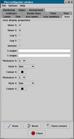
This page allows you to control whether axes lines are drawn around the plot or not. In general this isn’t very useful for spectral plots (when the outer border lines and axes are coincident), but it does allow you to draw the axes inside the display area and position where these are drawn, so you can define an arbitrary origin. Useful effects can then be obtained using grid lines.
The Log X: and Log Y: options are the same as those shown in the Limits pane.
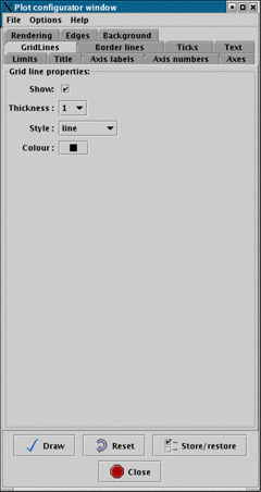
This page allows you to configure if grid lines are drawn in the plot, or not (not by default). Grid lines are drawn between the major ticks. You can also set the thickness, style and colour of the grid lines.
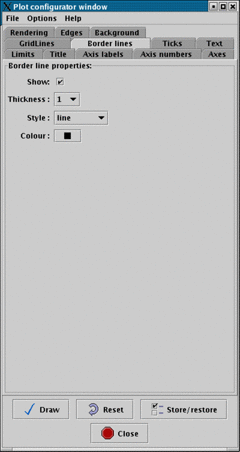
This page allows you to configure if border lines are drawn in the plot, or not. Border lines are drawn at the data limits of the plot. You can also set the thickness, style and colour of the border lines.
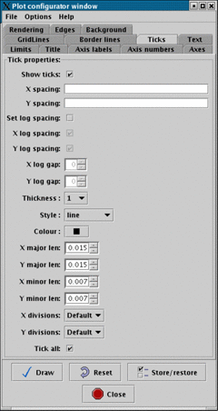
This page allows you to define whether to show major and minor tick marks or not. It also allows you to define the spacing between major ticks and the number of divisions (minor ticks plus one) between major ticks, as well as the properties of the tick lines and their lengths.
The spacing used between major ticks may be dependent of the number of significant figures used in the axis number labels, so you may need to also change that.
The option Set log spacing: together with X log spacing and Y log spacing allow you to define if the spacing of major ticks along an axis are logarithmic. If the axis is scaled logarithmically (that is you’ve asked for log axes in the data limits tab) then log spacing is the default, otherwise major ticks are spaced linearly.
When spacing logarithmically you can define the separation of the major ticks using X log gap: and Y log gap:. These values are the power of 10 you require between adjacent ticks, so for instance, if you wanted ticks every factor of you’d use .
This window has no uses in SPLAT-VO.
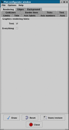
This page allows you to define how carefully the graphics are drawn in the plot display area. By default any text is drawn using anti-aliasing, which makes the graphics less jagged, and spectra are drawn without anti-aliasing. If you’d also like the spectra to be anti-aliased tick Everything:.
It’s not possible to anti-alias the spectra and not the text (so it’s not just a perverse choice of options). Also note that any rendering options are applied to any captured JPEGs produced in the plot.
Finally anti-aliasing is a CPU expensive procedure so it can result in a significant performance degradation (so the default is switched off for spectra).
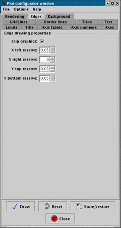
This page allows you to change the amount of space reserved around the plot for displaying titles and axis labels etc.
It also clips any points of any of the plotted spectra that lie outside the bounds of the data limits (this is not normally the case, unless you’ve defined data limits of your own).
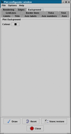
Use this page to select a colour for the background of the plot display area.
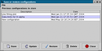
This additional window is activated by the Store/restore button. It’s purpose is to allow you to create a database of configurations that you’d like to keep (after all if you’ve spent some time configuring the look of a plot you don’t want to have to type it all in again when someone asks you to tweak the postscript).
The configurations are identified by two elements, a Description entered by you and the
date when the configuration was created. To create a copy of the current configuration
(note this doesn’t include the spectra themselves) just press the Store button. This creates a
new entry with the description New configuration. To change the description just double
click on this text and type in your changes. Remember to press <Return> when you’re
done. To remove any un-needed configurations select their rows and press the Delete
button.
To restore a configuration just select it and press the Restore button. The actual data is stored in the
file: $HOME/.splat/PlotConfigs.xml. If things seem badly broken then try deleting this
file.
This window is used to cut out or remove sections from the current spectrum. The sections are defined as a series of graphics ranges that you draw on the plot display area.
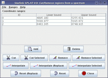
To add a region press the Add button and then drag out a region in the display area of the plot window. This should result in the creation of a green rectangular figure.
You can interact with the figure, moving it side-to-side and resizing it. To do this point at the figure
and press the left mouse button. This ‘selects’ the figure and adds grips to its exterior. Note that it also
becomes the selected row in the Coordinate ranges: table. To move the figure just drag it and to resize
it drag a grip (the little black squares). The associated coordinate range in the table updates with these
changes.
To add a second range just press Add and repeat. The ranges can be overlapped or not.
To fine tune the ranges you can edit the values in the ranges table, just point at the cell you want to
change and double click the left mouse button. This should enable the text editing cursor. Just make
the modifications you want and press <Return> to make the changes permanent. (Note: if your spectra
have sky coordinates shown for the X axis, then you should use the same format for your
edits).
To read a set of ranges from a disk file choose the File->Read ranges menu item. The format of the input file is simple. It should have two fields separated by whitespace or commas. Comments are indicated by lines starting with a hash (#) and are ignored.
When you’ve got the ranges that you want to extract, remove or replace by linear interpolation, press
one of various the Cut, Remove or Interpolate buttons. This creates and displays a new spectrum on
the global list called Cut <n> of <shortname>, that you can save to disk, or display in another plot
etc. To just extract, remove or interpolate, one or a subset of the ranges select the rows in
the ranges table and press the Cut Selected, Remove Selected or Interpolate Selected
buttons.
To clear the ranges press the Reset button, but note that this also clears any spectra that have been created on the global list. To keep these just close the window.
When interpolating you will often just want to see the resultant spectrum, so there is a special Interpolate (Replace) action. That performs the interpolation, removes the current spectrum and then displays the result of interpolation. To go back from this change use the Reset (Replace) button (only undoes one change).
Accelerator keys
The polynomial fitting window allows you to fit a polynomial of selected degree to various selected ranges of the current spectrum. You can select to use errors as weights for the fit and can save the fits on the global list as spectra in their own right. Fitting a polynomial is generally a pre-requisite to fitting spectral lines.
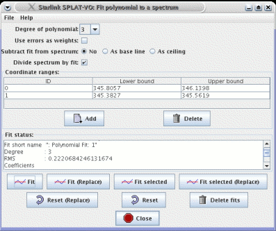
The Degree of polynomial drop-down list shows a series possible values for the degree of the polynomial that will be fitted. Obviously this should be chosen to match the expected complexity of the background.
The Use errors as weights checkbox is only effective if the spectrum being fitted has data errors.
The Subtract fit from spectrum series of radio buttons allows you to ask for the creation of a spectrum that is the difference between the spectrum and the polynomial fit. Use the As a ceiling option for absorption lines, and As base line for emission lines. These subtracted spectra appear on the global list and are added to the plot for display.
The Divide spectrum by fit checkbox allows you to ask for the creation of a new spectrum that is the
result of dividing the spectrum by the polynomial fit. You will probably want to do this before
attempting to fit absorption lines so that the continuum is normalized. The new spectrum appears on
the global list (with the name Ratio: <spectrum name> by <polynomial name> and can plotted in a
new window before fitting the lines.
Coordinate ranges
This part of the window is used to define the regions of the spectra that you want to fit the polynomial to.
To add a region press the Add button and then drag out a region in the display area of the plot window. This should result in the creation of a green rectangular figure.
You can interact with the figure, moving it side-to-side and resizing it. To do this
point at the figure and press the left mouse button. This ‘selects’ the figure and adds
grips to its exterior. Note that it also becomes the selected row in the Coordinate
ranges: table. To move the figure just drag it and to resize it drag a grip (the little
black squares). The associated coordinate range in the table updates with these
changes.
To add a second range just press Add and repeat. The ranges can be overlapped or not.
To fine tune the ranges you can edit the values in the ranges table, just point at the
cell you want to change and double click the left mouse button. This should enable
the text editing cursor. Just make the modifications you want and press <Return>
to make the changes permanent. (Note: if your spectra have sky coordinates shown
for the X axis, then you should use the same format for your edits).
To read a set of ranges from a disk file choose the File->Read ranges menu item. The format of the input file is simple. It should have two fields separated by whitespace or commas. Comments are indicated by lines starting with a hash (#) and are ignored. You can also save the ranges to disk (File->Save ranges).
When you’ve got the ranges that you want to fit, press the Fit button. This creates
a new spectrum on the global list, called Polynomial Fit: <n> and displays it in
the plot. You can save this to disk, or display in another plot etc., just like any other
spectrum. To just fit one or a subset of the ranges select the rows and then press the
Fit selected button.
To clear any fits created by this window press the Delete fits button. To clear the ranges from the display area and delete the fits press the Reset button. To keep any fits just close the window.
Fit status
The Fit status text area shows some facts and figures about the fitting process. The
RMS value is the root mean square difference between the fit and the spectra data i.e.:
Where and are the data values of the spectrum and the fit (possibly interchanged) and the number of positions in the spectrum.
Command Buttons
Accelerator keys
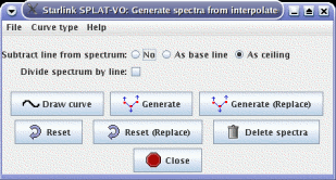
This window is for generating a spectrum that is equivalent to an interpolated line that you have drawn (or are about to draw) on the plot. Such lines can then be subtracted to or from, or divided into the current spectrum, thus providing a way to background correct a spectrum using a hand-drawn line.
Command Buttons
 option in the Graphics menu. Different
types of interpolated lines can be selected first in the Curve type menu. The default is
hermite a type of spline that attempts to connect points in a similar way to a hand-drawn
curve.
Accelerator keys
The spectral line fitting window allows you to measure the wavelength and equivalent width of emission or absorption lines and to fit various standard profiles to the lines.
The standard profiles offered are Gaussian, Lorentzian and Voigt, as well as a model independent intensity analysis measure.
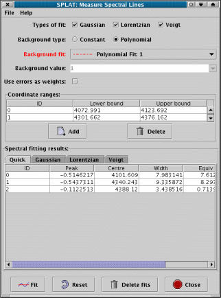
Background type: Choose a type of background estimate to be subtracted from the spectrum before fitting. The choices are Constant and Polynomial. If you have already subtracted the background from the spectrum, or have applied a normalisation (so that the background is flat, usually with a value of 1) then you need to choose Constant and provide a suitable value. Otherwise choose Polynomial and select a spectrum from the list in Background fit.
Background fit: For emission lines you would normally define a background spectrum using the polynomial fitting tool. In this case select the Polynomial option and choose the background spectrum you have created. Note that you can actually use any spectrum from the global list as the background (so you are not restricted to what SPLAT-VO, provides) but if you choose the same spectrum as is being measured then a background of is assumed.
The default background should be set to the first polynomial found on the global list.
Use error as weights: If your spectrum has associated error measurements then you can select this checkbox to use the errors as weights in the fitting procedure.
Coordinate ranges: This table shows the upper and lower coordinate range for each line that you want to measure.
To add a line to this list press the Add button. Now drag out a region on the plot display area that encompasses the spectral line. You should now see a yellow rectangle over the line:
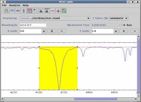
Note that the rectangle is just defining a range, not an area, so you just need to worry about its width and position along the X axis, not its height.
To adjust the rectangle position select it and either drag it around, or use the grips on the exterior to
resize it. You can see the physical extent of the region in the Coordinate ranges: table. To set these to a
known value double click on the value you’d like to set, make the change, and then press <Return> to
apply it.
The extents of lines can be saved to a simple text file and re-read. The format is simple. It should have two fields separated by whitespace or commas. Comments are indicated by lines starting with a hash (#) and are ignored.
Types of fit:
Once you have defined the extents of your spectral lines and chosen a background, you can proceed to make the measurements you want. Just select the types of fit you want from the list Gaussian, Lorentzian and Voigt. Note you can de-select all these and just get a Quick measurement.
All types except Quick use a non-linear least squares (Levenberg-Marquardt) minimisation stage to perform the actual fit of the model to the data (possibly with weighting, if the spectrum has any error measurements). So it is necessary to have some idea of the shape of the line, before attempting to fit it. This job is done by the Quick fit, which is compulsory. The description of each of the types and what their measurements represent is given below.
The error estimates are based on the variances produced by the fit. If you have errors for the data values, these will be used as weights and providing they are realistic the errors will be correct. In the absence of data errors the errors produced will be decided assuming that the fit is good (the chi-square statistic will be artificially forced to have a value of 1).
Quick: The default line measurement type. This is based on the ABLINE technique described in the FIGARO documentation. This just uses an analysis of the intensities in the selected region and the chosen background. The results you get are:
ID, just a unique integer to label the line. This is the same for all fits.
Peak, the peak, background subtracted, intensity in the region. Negative for
absorption lines.
Centre, the position of the median value i.e. that for which half of the total,
background subtracted, area of the line, within the given region, lies to the left
and right.
Width, width of the line. For a Gaussian this would be
standard deviations wide.
Equiv, the equivalent width of the line. This will be
if a zero background is given or assumed.
Flux, the background subtracted integrated intensity of the line over the
selected region. Requires a linear coordinate step.
Asym, an asymmetry value for the line. This is a measure of the relative
displacement of the centre of the line from the centre as measured by the upper
and lower half widths.Gaussian: The formula used for the Gaussian is:
where is the scale height, is the distance from the centre, is the centre, the distance from the origin and is the Gaussian sigma. The values are background subtracted.
The values measured for this line shape are:
ID, integer identifier (same as other fits).
Peak, the Gaussian peak ().
PeakErr, an estimate of the error.
Centre, the position of the Gaussian peak ().
CentreErr, an estimate of the error.
Width, the Gaussian sigma ().
WidthErr, an estimate of the error.
FWHM, the full width of profile at half maximum.
FWHMErr, an estimate of the error.
Flux, the integrated flux of the Gaussian.
FluxErr, an estimate of the error.
Rms, the root mean square difference between the Gaussian and the line data.Lorentzian: The formula used for the Lorentzian is:
where is the scale height, is the distance from the centre, is the centre, the distance from the origin and the Lorentzian width. The values are background subtracted. The full width half maximum () of the curve is:
The values measured for this line shape are:
ID, integer identifier (same as other fits).
Peak, the Lorentzian peak ().
PeakErr, an estimate of the error.
Centre, the position of the Lorentzian peak ().
CentreErr, an estimate of the error.
Width, the Lorentzian width ().
WidthErr, an estimate of the error.
FWHM, the full width of profile at half maximum.
FWHMErr, an estimate of the error.
Flux, the integrated flux of the Lorentzian.
FluxErr, an estimate of the error.
Rms, the root mean square difference between the Lorentzian and the line data.Voigt: The formula for a Voigt profile (a convolution of a Gaussian and Lorentzian) is:
where:
and
In these equations is the central wavelength, the distance from the origin, is the Gaussian width and the Lorentzian width. Which is complex to solve. However, if we take a complex variable , then the Voigt function is, within a scale factor (), also the real part of the complex error function:
which has been approximated by various numerical codes. Using this fact with a non-linear minimisation routine (plus some derivatives) is how SPLAT performs its Voigt fitting.
The values measured for this line shape are:
ID, integer identifier (same as other fits).
Peak, the Voigt peak ().
PeakErr, an estimate of the error.
Centre, the position of the Voigt peak ().
CentreErr, an estimate of the error.
Gwidth, the Gaussian width ().
GwidthErr, an estimate of the error.
Lwidth, the Lorentzian full width at half maximum ().
LwidthErr, an estimate of the error.
FWHM, the full width of profile at half maximum (estimate).
FWHMErr, an estimate of the error.
Flux, the integrated flux of the Voigt profile.
FluxErr, an estimate of the error.
Rms, the root mean square difference between the Voigt and the line data.The measurements, as shown in the Spectral fitting results: table can be written out to a text file. Just select the File->Save line fits item and either pick an existing file to overwrite, or enter a new file name. The format of this file is very simple, as shown by the following example (long lines are wrapped for presentation):
So each fit type has a section in which the results for each line are shown. Lines are
uniquely identified by their ID value.
Accelerator keys
This window provides the ability to filter the current spectrum displayed in a plot.
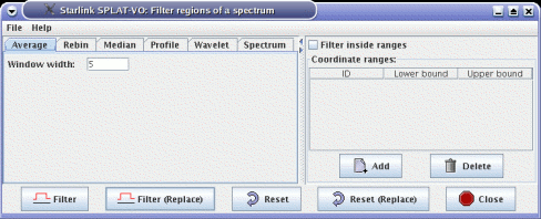
The various options are:
Average take the running average value over a number of positions.
Rebin rebin a spectrum so that one output value equals the mean of a number of input
values.
Median take the running median value over a number of positions.
Profile smooth the values using a profile matched to typical line shapes, Gaussian,
Lorentzian and Voigt and the standard Hanning, Hamming, Welch and Barlett filters.
Wavelet use various wavelet filters to convert the spectrum into multi-resolution
coefficients, removing a fraction of the coefficients, thus denoising the spectrum.
Spectrum smooth the values using a profile defined in another spectrum (allows you to
create kernels that match some shape, rather than just the standard profiles).You can define ranges of the spectrum to apply the filter over (except for Rebin, that always applies to the whole spectrum, which is what happens for all filters if you’ve not defined any ranges). Depending on whether you’ve selected Filter inside ranges or not the ranges are used to define the parts of the spectrum to filter, or not to filter. Parts which are not filtered do not form part of the result spectrum.
Command Buttons
Accelerator keys
This window allows you to change the coordinate or data units of the current spectrum to a limited number of preset values. You can only change units when the current spectrum already has a correctly set coordinate system or data units.
If you need to set the coordinates or data units you must use the two toolboxes available in the main window. These also offer considerably more flexibility, particularly when defining spectral coordinates.
If you do not want to change the units of an axis, just leave the value set at Not set or unrecognised.
When you see the value Not set or unrecognised, that means that the current spectrum has no properly defined coordinates or data units for that axis (as appropriate), or, that the settings do not match one of the pre-defined set that you can switch to. Note that data units which match one of the preset values dimensionally will be displayed in the preset format, so may not match values shown elsewhere, say in the plot labels.
When the plot is displaying more than one spectrum, only the current one is actually modified. If you want the other spectra to be drawn as if in the same coordinates or data units, then you must make sure that the menu item Options->Match coordinates and/or fluxes is selected, but this will only work when all the displayed spectra have proper spectral coordinates and data units defined.
The SideBand: control is for switching between sidebands (upper and lower) when display spectra that are derived from a dual sideband instrument. This is not available when your spectra do not have this feature. When displaying a dual sideband spectrum the inactive sideband coordinates will be displayed along the unused X axis (usually the top). You can also use this control to display coordinates offset from the Local Oscillator value.
The Origin: control allows you to display offset coordinates. In this case you can select to have no offset (None), use the existing offset, if defined (Default, usually the same as None), or display coordinates offset from the rest frequency. Note for velocities this last option isn’t useful as they are already displayed offset from this value. If you want to set another value as the origin then you need to use the advanced toolbox available in the main window.
The Standard of rest: control allows you to switch between the various supported rest frames. If the current spectrum doesn’t support these the value will be set to Not set or unrecognised.
The Rest Frequency: field displays the current rest frequency in GHz. This can be changed in two ways, either by selecting a position along the plot X axis, which you start by pressing the Pick pos button and then clicking on the plot, or by selecting a line identifier, which you do by pressing the Pick ID button and clicking on the plot in the vicinity of the desired label. When picking a line identifier the rest frequency is set to that of the line, not of the position that it currently occupies on the plot (these will differ if the spectrum has a source velocity).
Accelerator keys
This window allows you to do three related jobs.
Flipping and shifting a spectrum allows you to assess the symmetry of a line. Shifting alone to determine how well spectra are aligned and redshifting to transform a spectrum or set of line identifiers to guess or confirm the redshift (all line identifier lists are already editable).
The transformation is applied to the spectrum shown in the Spectrum: drop-down menu. Initially this will show any editable spectra displayed in the associated plot (like the line identifiers). If you want an editable copy of the current spectrum just press the Copy button.
One subtlety is that the offset value is either a redshift or a value in the coordinate units of the spectrum being modified, depending on whether the Redshift checkbox is selected, or not. The coordinate units of the spectrum may not be the same as those of the current spectrum in the plot, which can lead to surprising results.
When applying a redshift it is assumed that the spectrum being modified has a wavelength coordinate system, of some kind, unless it has a proper coordinate system defined. In this latter case the only restriction is that you cannot have a standard of rest set to ‘Source’ (as a transformation to and from Source is used to determine the redshift transform). In this latter case use the coordinate system toolbox to transform to another rest frame first.
The Reset button returns a spectrum to an offset of zero.
Visitor lists
It’s often the case that you have a list of lines, in a spectrum, or many spectra, that you’d like to step through to check the radial velocity or redshift estimates, without the bother of reading each spectrum and line, positioning the plot etc. That’s what a visitor list is designed for.
To use this create a simple text file containing either one, two, three or more whitespace separated columns. If one column is present then that is assumed to be the wavelength of the lines. If two columns are present then these are the wavelength and an associated spectrum. If three or more columns are present then the third columns contains the name of the associated spectrum and the second a label to be displayed at the position (when the label is missing it is set to the wavelength). Very short examples of the three types follow:
Visitor lists are a type of line identifier spectrum, so can have fully specified spectral coordinate units written in a header section (see the line identifier lists in the SPLAT distribution themselves for details), so you are not restricted to having all your spectra in the same coordinate systems.
Once the visitor list is loaded File->Read visitor line list, you can start stepping through it using the Visitor controls, or jump to a particular line using the drop-down menu. The default behaviour of this tool, on each visit, is to create a copy of the current spectrum and then flip it centred on the line (the current zoom is also preserved). It you’d like to not create a copy of the spectrum for each visit, or indeed to flip it, then uncheck the Flip checkbox and select the menu item Options->One spectrum for visitor (these choices remain enforced between sessions).
Another way to use the visitor controls is to use a line identifier (either a built in one, or one of your own) as the visitor list. To do this load the line identifiers in the usual way (in the main window) and display them in the plot. You can then make this the visitor list by pressing Set as visitor list. Now using the visitor controls you can step between the lines (remember to de-select Flip and select Options->One spectrum for visitor, otherwise you’ll get the line identifiers copied, flipped and maybe reused!).
SPEFO options
The original motivation for creating this tool (suggested by Petr Skoda, see the acknowledgements section) was really to do flip comparisons of lines to determine radial velocities in the same fashion as the SPEFO program. This has some additional requirements beyond those required for simple shifting in a linear sense, as well as in redshift, and are enabled by selecting the Options->SPEFO options menu item. This reveals two text areas (you need to resize the window to actually see them first time). The upper one shows the flip corrected offset (that’s half the standard shift) and the radial velocity for that flipped shift (calculated as ), assuming that the coordinate system is some wavelength.
There’s also an editable area for writing some notes about the measurement, both
these areas are written the file SPEFO.log by pressing the Save to SPEFO.log file
button.
Accelerator keys
Using this window you can get simple constantly updated statistics on regions of the current spectrum, or fuller statistics for the whole spectrum, or collections of regions.
Constantly updated statistics for regions are:
The integrated flux is a numerical estimate and does not require even coordinate spacing. It can be removed from this list by deselecting the Options->Show flux integral item. This can be used to quickly estimate the flux in a line, providing your spectra are background subtracted.
The TSYS value is a system temperature estimate and requires data from the JCMT, or you can set the necessary parameters by enabling the Options->Set TSYS parameters item, which reveals a set of controls not seen by default. Note that the effective exposure time is:
where and are the integration times spent on and off the source. The backend degradation factor is instrument specific.
When you use the buttons along the bottom of the window these statistics are extended to also include:
Note that the Mode is determined as , not from a distribution, so will not be correct for highly skewed distributions.
If you select the Options->Show extra stats menu item you can also see:
and if you select Error stats->you can get basic statistics on the values that are being used as the spectrum errors (or variances).
To get statistics for the whole of the current spectrum just press the Whole stats button. If you want statistics for parts of the spectrum you will need to define the coordinate ranges you want to use (see the next part), and then press the Selected stats button to get statistics for the selected regions combined together (if none are selected then all regions are used), or All stats to get statistics for all the regions combined together.
Coordinate ranges
This part of the window is used to define the regions of the spectra that you want to see statistics for. Once defined you will see simple, continuously updated, statistics. You can also get fuller statistics using the Selected stats and All stats buttons.
To add a region press the Add button and then drag out a region in the display area of the plot window. This should result in the creation of a green rectangular figure.
You can interact with the figure, moving it side-to-side and resizing it. To do this
point at the figure and press the left mouse button. This ‘selects’ the figure and adds
grips to its exterior. Note that it also becomes the selected row in the Coordinate
ranges: table. To move the figure just drag it and to resize it drag a grip (the little
black squares). The associated coordinate range in the table updates with these
changes.
To add a second range just press Add and repeat. The ranges can be overlapped or not.
To fine tune the ranges you can edit the values in the ranges table, just point at
the coordinate you want to change and double click the left mouse button. This
should enable the text editing cursor. Just make the modifications you want and
press <Return> to make the changes permanent. (Note: if your spectra have sky
coordinates shown for the X axis, then you should use the same format for your
edits).
To read a set of ranges from a disk file choose the File->Read ranges menu item.
The format of the input file is simple. It should have at least two fields separated
by whitespace or commas. Comments are indicated by lines starting with a hash (#)
and are ignored. You can also save the ranges and simple statistics to disk file using
(File->Save ranges). It is also possible to append the contents of the Full stats log:
region to the file SPLATStats.log by pressing the Save to log file button.
Accelerator keys
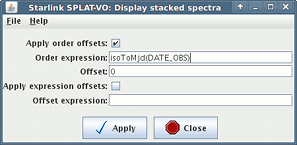
Using this window you can change the display of multiple spectra so that an offset in data value is artificially applied so that the spectra can be viewed stacked one above the other. It can also be useful when say comparing spectra from different times or physical state, as the stacking order can be defined as an algrebraic expression that can include time and dates or the actual offset as an expression of some other physical parameter, like period.
In both modes the offset is a value in the data units of the spectra, which must all be the same, no flux matching is supported.
If supplying an order expression it should evaluate to a number for each spectrum, higher values having their associated spectra placed above lower valued ones by the given offset.
If supplying a offset expression it should evaluate to a physical value, so scaling to appropriate values is often necessary.
Note that the values of any properties associated with the spectra are available for use as part of the expression, usually these are the values of the FITS headers and the keywords should be used.
The expressions are the same as used in the TOPCAT application (see SUN/253 or the TOPCAT builtin help), so include all the special functions it provides, for instance isoToMjd will convert an ISO 8601 date into an MJD, which is suitable as a order value. As an example the expression isoToMjd(DATE_OBS) will convert the DATE-OBS value into an MJD, provided the DATE-OBS value is in ISO 8601 format. Note that the minus sign in DATE-OBS has been changed into an underscore, that is deliberate. Any character in a keyword that cannot be a Java identifier will be converted into an underscore (allowed characters are any alpha-numeric, plus the underscore).
Accelerator keys